
The Point:
A new set of default parameters, named “CARBON“, has been developed that increases 13C signal strength for all signals relative to traditional parameter settings. Some signal intensities are DOUBLED relative to results obtained with commonly-used parameter settings in the same amount of experiment time. This is the result of careful optimization of key acquisition parameters, resulting with AQ=1.0, D1=2.0, NS=128, and P1=8.25 (on 400-1) with the pulse program zgdc30, which automatically multiplies P1 by 1/3. The whole experiment takes approximate 6.5 minutes. Best practice is now to use CARBON by default for most samples, increasing NS to intensify weaker signals, but NOT changing other parameters.
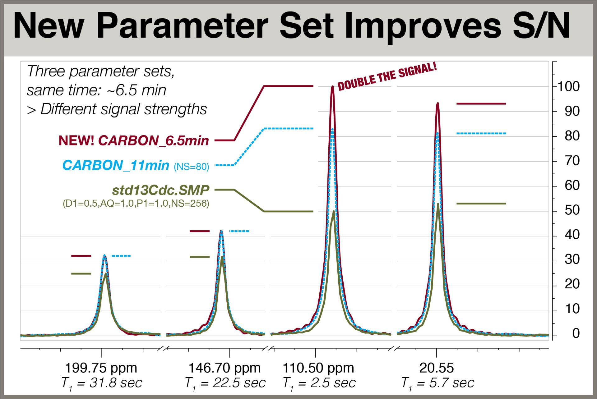
Fig. 1: Bottom line new method can double S2N
TLDR:
- The aim of optimizing 13C acquisition parameters is achieving the best overall signal-to-noise ratio (S/N) for the most peaks of interest in the least amount of time. Unlike 1H NMR, we are generally unconcerned about ensuring that integral values from different peaks can be compared.
- T1 relaxation values, which help optimize 1D experiment parameters, were obtained on a small set of molecules MW 150 – 180. Measured T1s ranged from 2.5 to 46 seconds.
- Because these T1 values are long compared to expected experiment time (D1+AQ), and because 13C signals practically always require NS>1, 90-degree excitation, which requires experiments with D1~5*T1, would never be a viable option for typical organic samples. Bruker systems are geared for precise automatic 30° excitation with the pulse program zg30 and its counterparts, so we assume we’ll use 30° excitation.
- Further, we know we need both 1H decoupling during acquisition and 1H irradiation during the relaxation delay to provide 1H-13C Nuclear Overhauser Enhancement (NOE, which can increase a 13C signal by as much as 200%). The common 30°-excitation pulse programs (PULPROG) that satisfy these needs are zgdc30 and zgpg30. P1, the excitation pulse width, can be set to its proper angle with the getprosol command/button/routine.
- Ernst Angle calculations, discussed in the previous blog post, indicate that for a 30° excitation and T1 of approximately 21 sec (which is in the middle of our expected range), the best value for D1+AQ is 3.0 sec.
- Acquisition time, AQ, appears best at 1.0 sec. Shorter values give rise to “ringing” distortions of the peak shapes due to signal truncation. Longer values do not benefit unweighted linewidth and have little benefit on S/N.
- 13C signals were enhanced by as much as 160% with 2.0 sec of NOE 1H irradiation. Noticeably greater NOE requires additional investment in time that would be better spent enabling more scans to be acquired. 1.0 sec of NOE still yielded as much as 120% enhancement, but, if paired with AQ=1.0, would no longer satisfy the Ernst Angle condition. If paired with AQ=2.0, 1.0 sec of NOE would simply not yield as much signal. Thus we set D1=2.0.
- Default processing parameters, usually set to EM weighting with LB=1.0 Hz, were changed to:
- SI=256K, to provide smooth lines via zero-filling
- A slightly shifted gaussian window function, WDW=GM, with LB=-0.2 and GM=0.07 to yield significantly narrower lines and slightly greater S/N. Note this requires processing commands “GF” and “GFP” instead of “EF” and “EFP”, respectively. See the comparison below.
DETAILS
T1 Measurements
To optimize the durations of the acquisition time, AQ, and relaxation delay, D1, it is essential to know what values of T1 are expected for the molecules of interest. Signals that take a long time to relax via spin-lattice mechanisms can be severely attenuated if the experiment time D1+AQ is too short. This is especially problematic because the weakest signals in 13C spectra are the ones that generally take the longest to relax, requiring the greatest experiment times D1+AQ. Because T1 relaxation mechanisms proceed mainly through 1H-13C interactions, methyl and methylene carbons have much shorter T1 values than, say, quaternary or ketone carbons. Further, the lack of bound 1H atoms means their intensities cannot be enhanced much by the 1H-13C NOE. Knowing typical 13C T1 values is thus key to parameter optimization.
13C T1 measurements were taken on three molecules: S-carvone, cis-2-methoxycinnamic acid, and (-)-alpha-thujone. The pulse program t1irig was chosen so 1H decoupling during acquisition would be performed, but NOE during the relaxation delay would be absent. The low sensitivity of 13C relative to 1H necessitated use of large number of scans per spectrum (e.g. NS=64) and only eight spectra with different interpulse delays to create the inversion-recovery buildup curves.
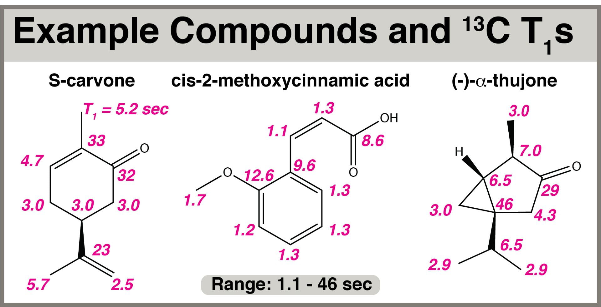
Fig. 2: Example compounds and their measured 13C T1 values
T1 values in these molecules ranged from 1.1 to 46 seconds. A target signal T1 of ~20 sec, in the middle of this range, was chosen for optimization to balance the need to observe low-intensity long-T1 signals with the potential for increasing intensity of shorter-T1 signals.
Optimal Pulse Program Choice
As discussed in the previous blog on optimizing 1H acquisition parameters, the most reliable pulse sequences that do not use 90° excitation are the ones that automatically divide the automatically-recalled, thus calibrated, 90° pulse by 3 to yield 30° excitation. Bruker has a family of such 1D pulse sequences, depending on whether and when the transmitter on the second RF channel is switched on. zg30 if the simplest pulse program, having no activity on the second RF channel. See the figure:
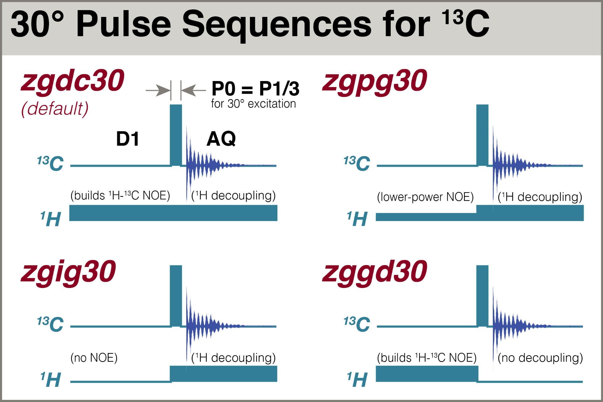
Fig 3: 30-degree 13C pulse sequences with 1H RF
For acquiring standard 13C 1D spectra, we need…
- 1H decoupling during acquisition (AQ) so the 13C signals all appear as singlets (except for those coupled to non-1H NMR-active nuclei, like 2H and 19F).
- 1H low-power transmission during the relaxation delay (D1) to provide 13C signal enhancement via the heteronuclear NOE.
Thus, we need a pulse sequence with 1H switched on during both D1 and AQ, and that limits us to zgdc30 and zgpg30. (There’s also a zgcw30, but it uses a very old scheme that is prone to heating the sample, so let’s not consider it.) The “pg” (power-gated) variety enables the NOE buildup to be accomplished at a lower power than the “dc” (decoupled). A test comparing performance of the two, including comparison of the rates for NOE buildup, yielded no significant differences (data not shown). We therefore choose the zgdc30 pulse program.
Ernst angle calculation
Recall the discussion of the Ernst Angle, which relates the sum of the D1 and AQ periods to the optimal excitation angle needed to achieve the strongest S/N in set amount of time, given a certain T1:
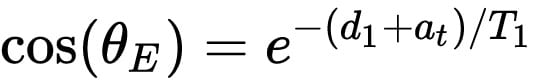
Fig6 The Ernst Angle equation
As described above, for general 13C 1D spectra, we should choose theta = 30° and T1 = 20. That yields D1+AQ = 2.87 sec. For ease, we can choose D1+AQ=3.0, making conditions optimal for signals with T1 = 20.8 sec, which should serve our purposes adequately.
Optimization of AQ
A special pulse sequence, zgdc30_sepnoe.jk, was created that divides the relaxation delay D1 into an NOE period, D8, preceded by a period where the transmitter is off. This enables D1 and AQ to be varied so their sum remains constant, but keeps the NOE period the same among experiments, thus enabling comparison for evaluation of best AQ.
We see in the next figure an overlaid set of spectra acquired with AQ values = 0.25 to 3.0, and processed with zero-filling to 512K points but no multiplication by any window function.
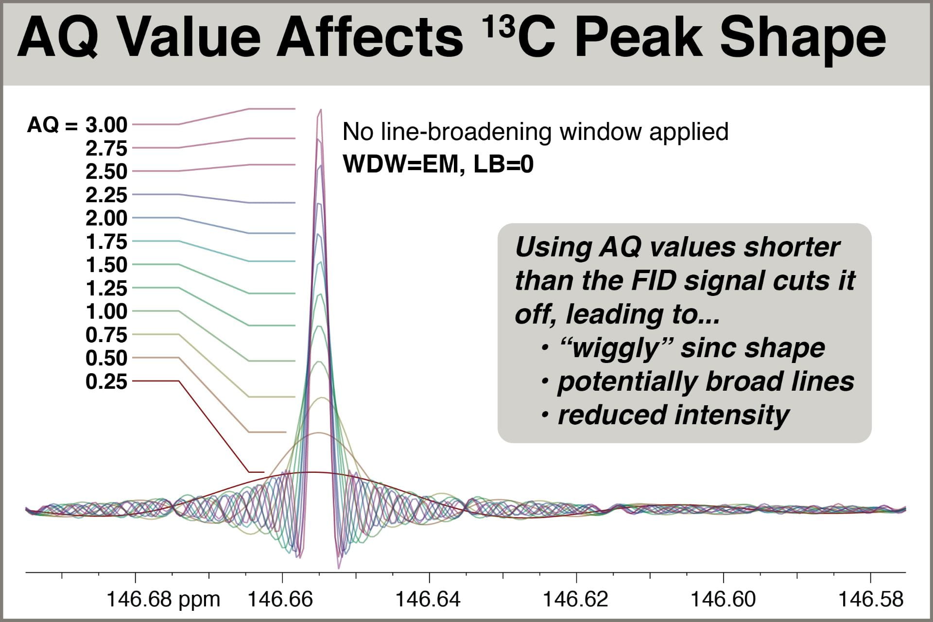
Fig. 4: AQ value affects 13C peak shape
NOTE ON THE WIGGLY SHAPE: One may be surprised at the distorted shape of the peaks when acquired using small AQ values. While we normally associate NMR peak shape with lorentzian functions, truncating the FID confers the addition shape of a sinc function, which has negative lobes an “wiggles“. The reason for this particular shape has to do with the math behind the Fourier transform (FT). Consider the everyday application of the EM (exponential multiplication) window to the time-domain FID that confers “line broadening” (LB) to the frequency-domain peaks. The FT of an exponential decay is a lorentzian-shaped peak; each NMR peak can ideally be considered a sine function multiplied by an exponential decay that yields a delta function (the FT of a sine function) multiplied by a lorentzian line shape. In the experiments above, we can consider the choice of a short AQ time to be like multiplying the time-domain FID by a step function, whose FT partner is a sinc function. While we only see this artifact sometimes in 1D NMR, usually around the sharpest peaks in the spectrum, it is quite common to see the effects of truncation in 2D spectra, where the indirect “FID” (interferogram) is extremely short – just 64-256 points, usually. The result is “T1 stripes” and “ridges” in the indirect dimension that sometimes exhibit 2D peaks in regular intervals corresponding to the crests and valleys of sinc wiggles.
As a practical matter, we can assume we will always multiply the FID with a window function.The most common is an exponental decay function (WDW = EM), the strength of which is determined by the parameter LB. For 13C signals, using LB = 1.0 offers a good compromise between reducing noise while retaining peak sharpness. Here we overlay the same peaks shown above, but with LB = 1.0 this time.
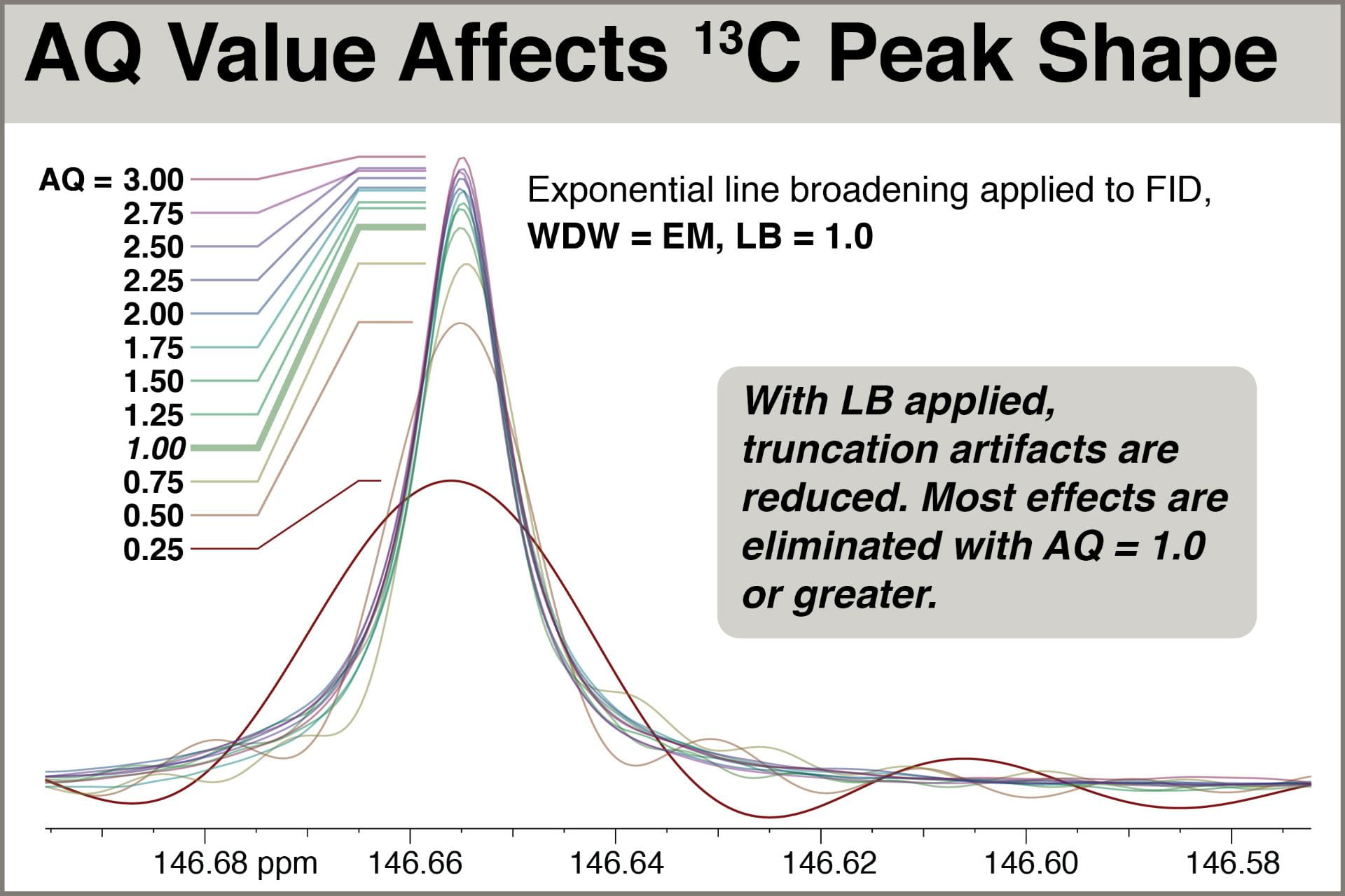
Fig. 5: Effects of AQ on 13C peak shape with LB=1.0
Examination of the overlaid spectra shows that use of AQ=0.25, 0.50, and 0.75 still give rise to fairly severe sinc distortion, even with LB=1.0. Spectra with AQ=1.0 and above, however, are relatively undistorted and all appear to have approximately the same natural linewidth. Peak intensity grows only slightly (~8%) with AQ longer than 1.0. Seeking to minimize AQ, thus helping satisfy the Ernst angle condition of D1+AQ=3.0, setting AQ=1.0 works well.
Insights into 1H-13C NOE, Optimal D1
Because 13C signals from most samples are weak, every “normal” 13C 1D spectrum boosts their intensity using 1H-13C Nuclear Overhauser Effect (NOE) (click here for a more detailed, yet readable, discussion of the relevant theory). In theory, the enhancement can be as strong as 199%, i.e. achieving 3X original intensity! In practice, the enhancement is highly variable, depending on the number of 1H signals near the carbon atom and other factors. Quaternary carbons, for instance, generally receive very little enhancement, whereas methyl carbons usually grow to over double their unenhanced size.
1H-13C NOE is effected by applying a series of low-power 1H pulses to the sample during the D1 relaxation delay (this is usually depicted by a simple low rectangle in the pulse sequence, not explicitly showing all the small pulses, see Fig 3).
Considering that the NOE is fundamentally a kinetic effect, we should ask, “For how long do we need to apply the 1H pulses during D1 to achieve good enhancement?” In principle, NOE buildup rates could be calculated using complex theory combined with 3D molecular modeling for a variety of molecules. Instead, let’s simply measure enhancement as a function of NOE irradiation time for all 13C signals in our small set of “typical” organic molecules, and then look for trends and potential correlations with 13C T1 values.
Using the aforementioned pulse program zgdc30_sepnoe.jk, a series of spectra were acquired with the same experiment time D1+AQ, but employing different durations of NOE, D8.
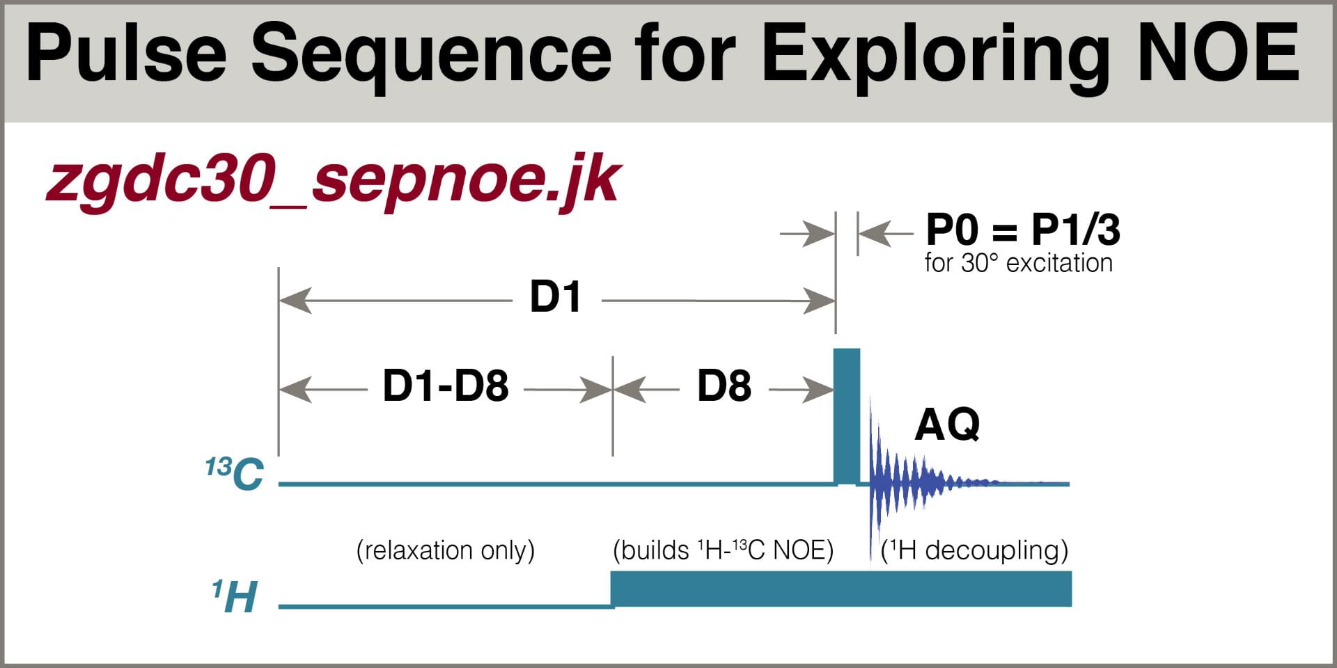
Fig 6: Special pulse sequence for exploring 1H-13C NOE kinetics
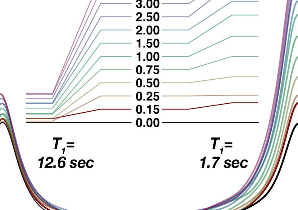
A series of 1D 13C experiments using this pulse sequence were acquired for cis-2-methoxycinnamic acid, which includes 13C signals bearing T1 values ranging from 1.1 to 12.6 seconds. For this experiment, AQ = 2.0 sec and D1 = 6.0 sec to ensure results would not depend significantly on total relaxation time AQ+D1. D8 values were set to 0.15, 0.25, 0.50, 0.75, 1.0, 1.5, 2.0, 2.5, 3.0, 4.0, and 5.0 seconds.
We can see the effects of the buildup qualitatively in the figure below showing overlaid peaks, and quantitatively in the accompanying chart.
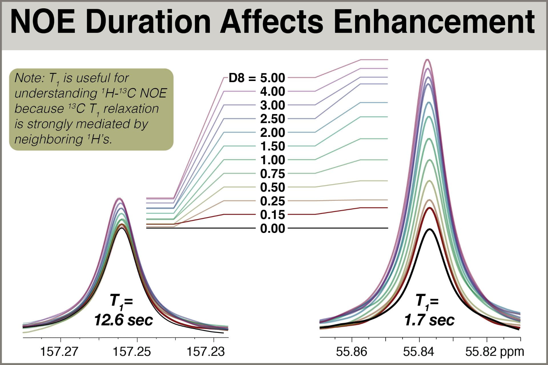
Fig 7: NOE duration affects 13C intensity, depending roughly on 13C T1
The data clearly show that NOE can be dramatic, but it takes time to build up. So why don’t we just use a very long NOE period like 5.0 sec to get maximum enhancement every experiment? Because that can dramatically lengthen each scan, lengthening total experiment time and/or reducing the number of scans we can acquire in a given time. So what would be the best NOE length, given the other constraints? To look at this more quantitatively, let’s plot signal intensity as a function of NOE duration to see just how quickly it builds up.

Fig. 8: Buildup of 1H-13C NOE
Rough examination of the shapes of the curves yields some practical insights. 1H irradiation provides different levels of NOE to different 13C atoms, and the effect is correlated with 13C T1 (long T1 correlating with little NOE). This correlation arises because 1H-13C NOE and 13C T1 relaxation utilize related mechanisms. Most signals studied achieved roughly maximum enhancement with 3.0 seconds of 1H irradiation, and 2.0 seconds provided almost all of the possible enhancement. Up through 2.0 seconds of irradiation, enhancement increases rapidly, and there are significant differences between 1.0 and 2.0 seconds of irradiation. The short-T1 carbon in this system goes from roughly 120% enhancement with D8=1.0 to perhaps 160% with D8=2.0. But the peak with slightly long T1, 1.7sec, benefits even more, going from ~80% to ~125%. That extra second yields an extra gain of 45% intensity for that peak.
Is relative gain resulting from 2.0 seconds over 1.0 seconds irradiation worth the extra time, relative to the benefit of increasing the number of scans afforded by a shorter experiment time D1+AQ? Let’s run a rough calculation with two models. Model A uses D1=1.0 (all NOE) and AQ=1.0, with 128 scans; total time = 256 sec. In the same amount of time, Model B uses D1=2.0 (all NOE) and AQ=1.0, with (256/3.0) 85 scans. Ignoring Ernst angle effects and NOE, the extra 43 scans in Model A should improve S/N by a factor of √(128/85) = 1.23, or 23% gain for the same total experiment time. But we’ve already shown the NOE effects bring a gain of 45%, making the extra second worth it. An NOE period of at least 2.0 seconds is thus called for.
Because we’ve already established using Ernst angle calculations that we’re aiming for D1+AQ=3.0, we can conclude the best D1 is 2.0 seconds, with 1H irradiation on during the entire period to build NOE.
Incidentally, many users employ the parameter set “std13Cdc.SMP” on 400-1, changing parameter values to D1=0.5, AQ=1.0, and P1=1. We can see in these NOE buildup graphs that D1=0.5 does not allow the NOE to build up to its full potential – just about 40% enhancement for a signal with T1 of 1.7 sec. While the very small tip angle resulting from P1=1.0 (~11° on 400-1) works well with the short D1 on an Ernst angle basis, the loss of NOE leads to a suboptimal level of signal enhancement.
Overall Comparison
Let’s compare the different major parameter sets using S/N measurements of key peaks with a range of T1 values. First, consider that to evaluate parameter sets on their ability to deliver the most signal in a given period of time, it’s important that all spectra in the comparison have approximately the same total experiment time. This involves changing the number of scans, NS, which, for practical reasons, makes it difficult to compare spectra by overlaying them. We therefore explicitly calculate the S/N value of each peak in each spectrum. Using the “SNR calculation non-interactive” tool in Mnova (noise region of 6000 points), S/N values were computed for four peaks in each of three 13C spectra of S-carvone acquired with the parameter sets shown in the following table. All spectra were acquired with total experiment times of 6 min 30 sec to 6 min 45 sec, and processed with zero filling to 512K and LB = 1.0 Hz. Once clearly sees the that CARBON parameters offer the highest S/N in the same amount of time for most peaks. The long-T1 peaks at 199.7 and 146.7 are approximately the same with the CARBON and CARBON_11min* (NS=80 so total time = 6:40) parameters.
| Parameter Set | Params | 199.7 ppm T1 = 31.8 sec |
146.7 ppm T1= 22.5 sec |
110.5 ppm T1= 2.5 sec |
20.5 ppm T1= 5.7 sec |
| CARBON | D1=2.0,AQ=1.0 zgdc30, NS=128 |
91.7 | 120.96 | 287.1 | 267.7 |
| CARBON_11min* | D1=3.0,AQ=2.0 zgdc30, NS=80 |
93.2 | 121.2 | 240.4 | 236.1 |
| std13Cdc.SMP | D1=0.5,AQ=1.0 zgdc, P1=1.0, NS=256 |
71.1 | 90.0 | 143.9 | 150.5 |
The S/N values shown here were used to manually scale the overlaid spectra in Fig. 1 above.
REAL-LIFE EXAMPLE
Recently, a user of 400-1 was found to be struggling to obtain a 1D 13C spectrum of a low-concentration sample. After an initial attempt of acquiring a sub-10-min spectrum with “traditional” parameters failed, a second attempt with additional scans was submitted with NS=2048 so the total experiment time would be slightly over 53 minutes. To test the benefits of the new parameter set, another experiment using the “CARBON” parameter set was queued for acquisition immediately after the traditional acquisition, editing only the NS value so the total experiment time would be about the same (slightly under 53 minutes). One further difference is the application of a resolution-enhancing gaussian window function to the FID of the data collected with new parameters; this was shown to have little effect on S/N, but markedly improved peak shape. The two spectra are compared here (key details omitted to obscure the nature of the sample):
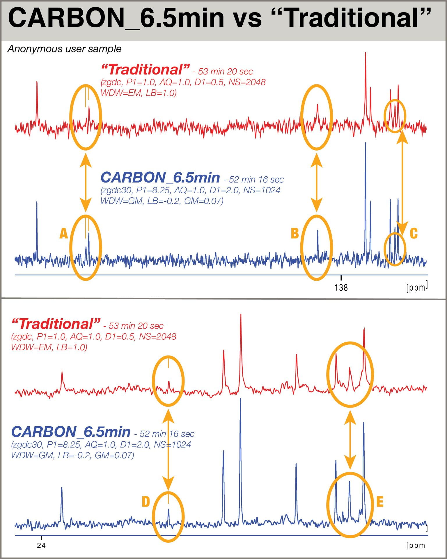
Fig. 9: Real-life comparison of parameter sets
Examination of the stacked spectra reveals key differences. In regions A and D, the “Traditional” parameters yielded signals difficult to distinguish from noise in regions A and D; one potential signal even appeared to the side of the larger peak in A that is not suggested in the “Traditional” spectrum. Peak B is clearly presented with greater intensity with the new parameters. The closely-spaced peaks in C and E clearly benefit from the greater resolution afforded by the application of the gaussian window. Acquired in the same amount of time as the “Traditional” spectrum, the spectrum employing the new parameters provided significantly more useful data.
CONCLUSION
Please enjoy CARBON the next time you need a routine 1D 13C spectrum. For dilute samples, the CARBON_3.5hr night-time 400-1 experiment now uses these parameters, but with NS=4096. If you have a moderately dilute sample, please use these parameters and change NS to whatever you feel appropriate, but do not change the other parameters, aside from the offset O1P and SW.
in your parameter set table you wrote zg30 and zg for pulse program.
i guess you have used zgpg30 and zgpg instead.
is this correct?
Thanks, Martin. I’ve fixed it, though I’ll mention I’ve usually used zgdc30 for 13C. I should probably switch to pg, though. I’ve recently been thinking about revisiting my default parameters again and lengthening the D1 delay to allow for more relaxation, in which case the “pg” will help reduce sample heating.
– Josh