
The Point:
Everyday 1H NMR spectra should be acquired with default parameter sets; that’s the whole point of having them. Most data can be acquired in one scan (params = PROTON1). If you want more than one scan, you should use PROTON8, even if you’re going to change the number of scans (NS). PROTON1 and PROTON8 use different pulse sequences, and the difference will affect your data.
This blog post goes into detail about how the important default 1H 1D parameters are set and why.
TLDR:
- For most regular organic samples, the PROTON1 parameter set works very well. One scan with 90° excitation yields plenty of signal, and the long D1 (17sec on 400-1) ensures good integrals.
- If you want more scans, please consider what you’re trying to accomplish.
- Want to reduce artifacts from vibration and other noncoherent sources? NS >1 does do that.
- Want to improve spectrum resolution? NS > 1 has NO effect – that’s nonfactual lab lore.
- Want to make signals appear stronger relative to noise? The effects are limited. To increase your S/N by a factor of two, you need to increase NS by a factor of FOUR – that’s an experiment four times as long. And then you need to consider quantitative factors of scan repetition.
- If NS > 1 is going to be useful for you, use the parameter set PROTON8, which uses 8 scans.
- The pulse sequence used here is different: is uses a 30° excitation instead of 90°; don’t touch P1.
- The parameter set “PROTON32” wasn’t getting much adoption; people seem to prefer 8 scans.
- If you need to enhance weak 1H signals (like end groups on a polymer), use PROTON8, and edit the NS value to something large, like 128 or 256.
- If you’re editing parameters every time you submit a sample, you’re wasting your time. Try these parameter sets out; if they’re not working for you, we can develop custom parameter sets for you.
- New default parameters:
- PROTON1: NS=1, AQ=3, D1=17 (400-1) / D1 = 5 (others), O1P=7, SW=16, PULPROG=ZG (90deg excitation)
- PROTON8: NS=8, AQ=3, D1=1.5, O1P=7, SW=16, PULPROG=ZG30 (30deg excitation)
DETAILS:
Background:
Even for the most common needs, such as 1D 1H spectra, setting default acquisition parameters can be a challenge. Assumptions must be made about what “typical” sample molecules are, what their sample concentrations are, and how much time users will accept for data acquisition. NMR theory only provides limited guidance, and a practical approach for development is merited.
Key real-world factors to consider:
- S/N (signal-to-noise ratio). Unlike UV/VIS spectra (for example), NMR spectra don’t generally have a meaningful scale on the vertical axis. Signal strength must be measured by comparing it with the level of noise in the spectrum.
- Though integrating peaks is straightforward, how does one “integrate” noise? In principle, noise should be equally positive and negative if sampled sufficiently. For the purpose of calculating a noise level, the software computes the “root-mean-squared” (RMS) noise – the numerical intensity of every point in a designated noise range is squared, then the average value computed, then the square root of the average is taken.
- A signal-to-noise ratio can then be calculated by taking the integral of a peak and comparing it to the RMS integral value of a specified region of noise.
- Signal intensity. When comparing spectra, it is often sufficient to simply overlay them and examine the height of the peak (the “signal intensity”), not necessarily measuring the integrated intensity.
- Total experiment time. Whatever NMR parameters are used, your primary interest is probably obtaining the most signal with meaningful intensities in the least amount of time. It turns out this is complicated, depending on several different parameters AND the particular sample.
- T1 Relaxation time. The apparent rate of decay you see when looking at an FID is called T2*, but the decay rate that affects how quickly spins actually relax back to equilibrium is called T1. T1 is a physical constant determined by a number of different factors, and these factors are different for every nucleus in a molecule. T1 values range from 0.2 to 3.0 seconds for most 1H signals in small molecules (MW 100 – 600), but T1 values of residual solvent signals are much longer – typically 10 to 60 seconds or more.
- Parameters over which you have control
- AQ: The time spent acquiring each scan of your data. This value should be determined by the time it takes for most signals to visibly decay, T2*. As a practical matter, default processing includes a “line broadening” factor, LB = 0.3 Hz, which has the effect of simulating the acceleration of signal decay, and setting AQ longer than ~3 seconds has little practical benefit. Thus, most 1H spectra use AQ = 3.0.
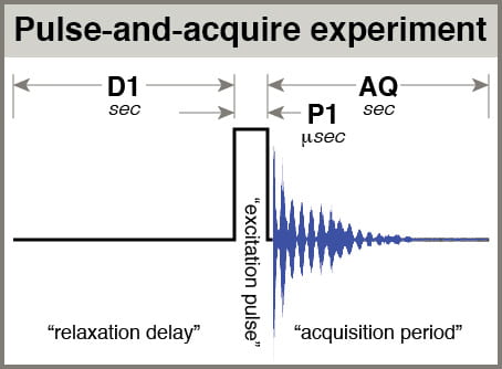
Pulse-and-acquire NMR experiment
- NS: The number of scans you’ll add together to get your final spectrum. Your main choice is whether to use NS = 1 or NS > 1.
- The intensity of each points in a peak should add constructively (1+1=2), but points in noise regions, being randomly composed of positive and negative points, should add semi-constructively (1+1 “=” √2). Accumulating scans thus adds more signal than noise, improving your signal-to-noise ratio, S/N. Ideally, increasing NS=1 to NS=4 should double your S/N.
- Using NS > 1 has the additional effect of reducing artifacts that appear with random phase, such as side-bands arising from sample vibration.
- For most non-polymeric organic molecules, NS = 1 gives sufficient signal.
- Use of NS > 1 requires consideration of the effects of repetition, which must factor in the T1 values in the molecule of interest.
- D1: the delay before your pulse. When considering relaxation of your spins, think about them being excited by your pulse, then relaxing partway during the acquisition period (AQ), then relaxing further during D1 before being pulsed again. D1 is referred to as the “relaxation delay”. The total amount of time you give spins to relax after being pulsed is AQ+D1. In a multiscan experiment with NS scans, the total experiment time is approximately NS * (AQ+D1).
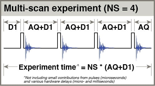
Multi-scan experiment
- PULPROG: ZG or ZG30 for 1H. You generally don’t set this yourself; it’s tied to the parameter set. When selecting the PROTON1 parameter set, the pulse program ZG is employed. When selecting the PROTON8 parameter set, the pulse program ZG30 is employed.
- “ZG” uses a 90° pulse for excitation, which is great for getting the most signal in one scan, but requires more time for relaxation before pulsing again. It’s used in PROTON1, but it should not be used for multi-scan acquisitions.
- “ZG30”: uses a 30° pulse for excitation, which is best if your NS > 1.
- Because it only excites your spins to 50% intensity per pulse, you don’t need to wait so long for your spins to relax back to equilibrium.
- TRICKY: the P1 value you see in the parameters still corresponds to the 90° pulse width; ZG30 automatically multiplies this value by 1/3, so the ACTUAL pulse width is NOT P1.
- ANY 1H acquisition with NS > 1 should use the ZG30 pulse sequence, so start with the parameter set PROTON8 and changes the NS value.
- P1: The 90° pulse width. All Bruker pulse sequences assume P1 corresponds to the pulse time required for maximum excitation – the “90° pulse width”. This is specially calibrated for each probe on each spectrometer for a particular power level, and the values cannot be interchanged. Setting “P1 = 3.0” or “P1 = 1.0” has no particular physical meaning. It is best to leave P1 alone unless you have a specific reason to change it and you know what you are doing.
- Setting P1 manually with the pulse sequences ZG30 and ZGDC30 can result in very low signals. If you try setting your pulse to give you a 30° excitation, for instance, you’ll actually get a 10° excitation, which is very small.
- AQ: The time spent acquiring each scan of your data. This value should be determined by the time it takes for most signals to visibly decay, T2*. As a practical matter, default processing includes a “line broadening” factor, LB = 0.3 Hz, which has the effect of simulating the acceleration of signal decay, and setting AQ longer than ~3 seconds has little practical benefit. Thus, most 1H spectra use AQ = 3.0.
Parameter Optimization
To make the default parameter sets best for everyone, let’s start by making some assumptions, then testing out the effects of various choices.
Guiding principles
- Spectrum S/N should be maximized in the least amount of total experiment time.
- Artifacts should be minimized.
- Integral values should be reliable for all normal sample peaks.
- Integral values for solvent, TMS, residual water, etc. should be ignored.
- Assumptions about “normal” samples:
- Molecules have MW ~80 – 300 g/mol
- Samples have ~10-20 mg compound
- Sample purity is irrelevant for parameter determination
NS=1 : No need for test
The best way to get good integral values is to wait an infinite amount of time, then excite spins with a 90° pulse. These conditions are practically produced using a single scan preceded by a long delay (e.g. 17 sec). These are embodied in the PROTON1 parameter sets.
TEST: Vary D1 with NS=8, 90° pulse excitation
To test the effects of different D1 settings on spectra, consider arrays of experiments with 90° excitation, 8 scans with AQ = 3.0 sec, and different D1 settings. In all the experiments shown here, fifteen D1 values were used:
D1 = 30, 20, 15, 10, 8, 6, 5, 4, 3, 2.5, 2.0, 1.5, 1.0, 0.75, 0.5 seconds
Here we see how the intensity of the residual DMSO-d5h signal depends on the D1 setting:

Fig3. 90° pulse excitation, NS=8, effects of D1 settings on residual DMSO peak
Obviously, the intensity of this peak depends very strongly on the D1 value. We therefore cannot use either peak height or peak integral values quantitatively for this peak unless we use an extremely D1 setting (e.g., 90+ sec).
Is it so bad for signals with shorter T1 values? Let’s see, for the molecule cis-2-methoxycinnamic acid:

Fig4 90° pulse excitation, NS=8, effects of D1 settings on peak with normal T1.
Under these circumstances, signals with “normal” T1 values aren’t strongly affected by D1. This depends HIGHLY, however, on setting AQ=3.0 seconds. Remember, the reliability of the integral values depends on the SUM of AQ+D1; the smallest recycle delay (AQ+D1) we’ve tried here is 3.5 seconds. If we had set AQ=1.0, the smallest total recycle delay would have been 1.5 seconds.
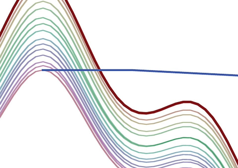
What about peaks with moderate T1 values? T1s of 2.0 – 6.0 seconds are common for aromatic, acid, and amine 1H signals, for instance.
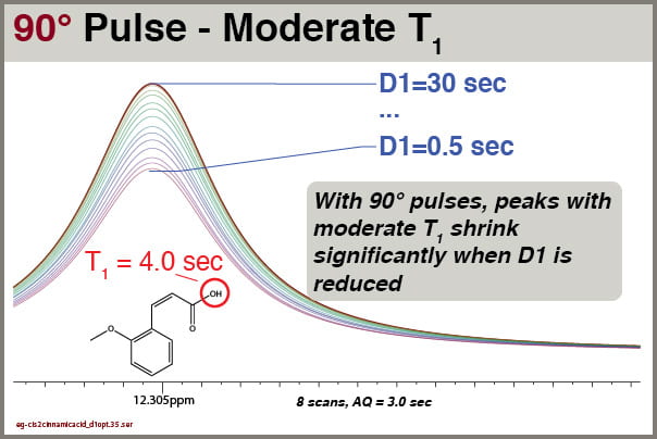
Fig5 90° pulse excitation, NS=8, effects of D1 settings on peak with moderate T1
The data show that peaks are moderate T1 (e.g., 4.0 seconds), shrink significantly when D1 is reduced. To ensure reliable integrals of these peaks with a 90° excitation pulse and multiple scans, one would need to set D1 to over 6-8 seconds. Such settings would make these simple routine spectra time-consuming and therefore costly.
CONCLUDE: Maybe the combination of 90° excitation and multiple scans (NS >1) isn’t worth it.
The Ernst Angle
The question of how to maximize NMR signal intensity in the shortest amount of time has been around for decades. Nobel laureate Richard Ernst approached this mathematically and derived an equation for the “Ernst Angle” – the excitation angle that will give rise to the most intense signal in the shortest time when doing signal averaging. It’s given by this equation:
Fig6 The Ernst Angle equation
Where Theta-E is the optimum excitation angle, d1 is the relaxation delay D1, at is the acquisition time AQ, and T1 is the T1 relaxation time of the peak in question.
BONUS: Check out who wrote a lot of this Wikipedia article.
LIMITATION: The Ernst angle can only be calculated for a single peak, so even if one peak is optimized, its integral value is not going to be quantitatively comparable to those of peaks with different T1 values from the same molecule. When setting default acquisition parameters to provide reliable relative integral values, we must therefore use the Ernst angle only as rough guidance, and consider the peaks with the longest T1s we can expect.
Example: For our peak with T1 = 4.0 sec, if we use AQ=3.0 and D1=3.0, the Ernst angle will be 77°.
Bruker’s Approach
As a practical matter, the excitation angle isn’t a great parameter to try optimizing for routine 1D work. It’s given by the pulse width, P1, and must be carefully calibrated differently for every probe on every instrument.
A better approach is to take advantage of the pulse sequences provided by Bruker that read the calibrated 90° pulse widths stored for each probe on each instrument, and multiply those values by 1/3 to achieve 30° pulses. If you open up a 1D 1H spectrum in Topspin, you can see whether you used a 90° excitation or a 30° excitation by looking for the parameter PULPROG or examining the tab labeled “pulseprog”; If you didn’t edit P1 and you used “zg”, you got a 90° pulse; if it was “zg30”, you got a 30° pulse.
If you assume a AQ=3, and D1=3, you can calculate that a 30° excitation is optimal for signals with T1 of 42 seconds – very long! Because most of our typical 1H signals have T1 much less than that, we can safely reduce our D1 value if we employ a 30° excitation.
Test: Vary D1 with 30° Pulse Excitation, NS = 8
Let’s explore how intensities of different signals respond to different D1 values when excited with a 30° pulse (pulse program = “zg30”). Like the examples above, we’ll use cis-2-methoxycinnamic acid, NS=8 and AQ=3.0
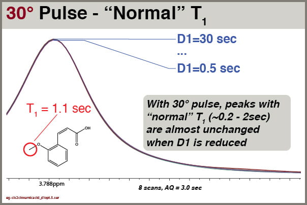
Fig7 30° pulse excitation, NS=8, effects of D1 settings on peak with “normal” T1
With a 30° excitation angle, we see the peak intensities are virtually unchanged by D1. We can thus get good integrals for most peak with even very short D1 values (e.g, 1.0 sec).
Consider the effects on peaks with moderate T1 values.
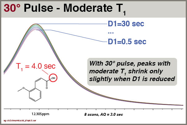
Fig8 30° pulse excitation, NS=8, effects of D1 settings on peaks with moderate T1
Even employing 30° excitation pulses, we still see some reduction of the intensity of peaks with moderate T1 values. However, the effects are relatively small. For this peak with T1 = 4.0 sec, we can quantify the peak height as a function of D1 setting:
D1 = 30, I = 100%
D1 = 5.0, I = 98.2%
D1 = 4.0, I = 97.7%
D1 = 3.0, I = 96.9%
D1 = 2.5, I = 96.4%
D1 = 2.0, I = 95.9%
D1 = 1.5, I = 95.1%
D1 = 1.0, I = 94.4%
D1 = 0.75, I = 93.8 %
D1 = 0.50, I = 93.1%
Of course, we want to choose the shortest D1 value that still gives us good integral reliability for peaks with T1 values we can expect to encounter.
In this test using 30° excitation, we see that setting D1 = 1.5 sec reduces peak intensity of a moderate-T1 peak by less than 5%, so that is the value now used as default in the PROTON8 parameter set.
Followup: how does varying D1 affect long-T1 solvent peaks with a 30° excitation pulse?
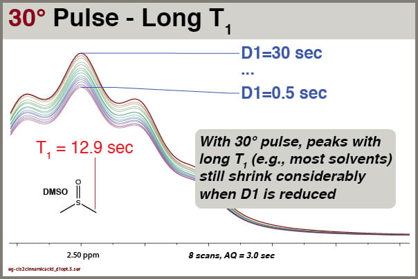
Fig9 30° pulse excitation, NS=8, effects of D1 settings on peaks with long T1 (solvent)
We see clearly that this solvent signal, with T1 of 12.9 sec, is still significantly affected by reductions in D1, even though excitation is accomplished with 30° pulses. You cannot rely on integrals of solvent peaks to be quantitatively meaningful. NEVER use residual solvent peaks to measure concentrations!
CONCLUSIONS
- For most samples, the best 1D 1H parameter set is PROTON1 (one scan, 90° pulse)
- If multiple scans are desired, use PROTON8 (30° pulse, 8 scans but NS can be changed if desired)
- AQ = 3.0 in both parameter sets to provide good resolution without acquiring excessive noise.
- D1 = 1.5 sec for PROTON8 to minimize total experiment time while retaining 95% peak intensity reliability for most sample peaks.
- Don’t change P1.
- D1 for PROTON1 is longer on 400-1 than on manually-operated instruments to provide extra time to make automatic gain adjustments.