

SUMMARY
Short instructional videos for how to perform a 1D NOESY experiment are now posted on the new NMR Facility YouTube channel:
https://www.youtube.com/channel/UCXv120eTmLYky1tOjyCraRg .
They are entitled
• “How to set up 1D NOE on one peak” (2m25s) and
• “How to set up 1D NOE on multiple peaks” (4m26s).
Point-of-use Learning
At each of the 500 MHz instruments, you will now find a small sign showing a QR code for each video. When you want to run a 1D NOESY, simply walk up to the spectrometer and use your phone to read the QR image, follow the link that comes up, and watch the step-by-step video (you can pause, go back, scan forward, and do whatever else you need). Once you watch the process, you’ll see that it’s very easy. On an iPhone, simply open your Camera app and point it at the QR image; a link will pop onto your screen, and when you tap the link, the video will open in YouTube. Something like that should work for Androids as well.

Where to find QR codes at the spectrometer computer
Why NOESY?
Please recall that the 1H-1H NOESY shows which hydrogen atoms are close together in space (under 4 or 5 Å), regardless of the chemical bonds between them. It’s good for answering qualitative structural questions like “is this H axial or equatorial?” and “which of these geminal vinyl Hs corresponds to which NMR multiplet?” It can also be used for structure determination, including quantitative 1H-1H distance measurement (if done carefully). It can even be used to determine forward/backward rates for systems in equilibrium on the 0.1 – 5 second timescale (NOESY is called EXSY when used for this purpose).
Key NOESY Facts
- 2D NOESY can be run without significant user intervention, but 1D NOESY requires manual selection of one peak for excitation. Oftentimes one runs sets of 1D NOESY spectra, selectively exciting several peaks in separate experiments.
- 2D NOESY experiments generally run ~2.5 – 12 hours on typical organic samples, but 1D NOESY experiments can yield significant results in about ten minutes.
- 1D NOESY spectra of small molecules are displayed with the large excited peak phased negative and the NOE peaks phased positive.
- NOE peaks are weak – typically less than 2% of the intensity of the excited peak, often as little as 0.01%. It is worthwhile to take as many scans as possible to reveal weak NOE peaks.
- NOESY experiments always include a kinetic aspect. The NOE builds up during a delay in the experiment called the “mixing time”. By convention, this delay is D8 in Bruker pulse sequences. It is typically set to around 600 msec for small molecules.
- Magnetization transfer by NOE between spins can be quantified. NOESY with D8 of just 10 msec (very short) yields almost no magnetization transfer, so the integral of the excited peak in this 1D spectrum can be used for quantitative reference when compared to peaks in spectra acquired with the same parameters (but longer D8 values).
- Internuclear distances can be measured quantitatively in Å if calibrated with a 1H-1H pair of known separation. The NOE is VERY sensitive to distance; large NOE values for close protons drop in proportional to 1/r6 as distance grows:
runk = rref * (NOEref / NOEunk )1/6 - NOESY spectra often contain artifact peaks in which multiplets have both positive and negative peaks. These are known as “zero-quantum coherence artifacts”. Though they look like they interfere, they integrate to zero across the whole peak, and oftentimes do not affect quantitative measurements.
- NOE intensity varies with molecular weight because size affects the rate of molecular tumbling. Unfortunately, molecules with MW near 600-900 can tumble at rates that give rise to small or even zero NOE no matter how close the H atoms are. Rotating Frame NOESY (ROESY) offers an alternative for these systems.
Method
Step 0: Sample prep
NOE signals are inherently weak (typically ~0.1-1.0% of regular peaks), so make sure you have a reasonable amount of material for answering the question at hand. For reference, this blog post uses data taken on a 10 mg / 1 mL sample of carvone (MW 150). It’s best to use a good NMR tube for the best shimming; bring out the trusty Wilmad 528-PP from the velvet-lined box you keep for your personal special tubes.
Some texts suggest you should degas your sample to remove O2, which is paramagnetic and promotes spin relaxation. Degassing is best practice if you’re doing very careful absolute distance measurements, but most questions can be answered without it.
Step 1: Acquire a 1D 1H spectrum
Nothing special here. A default Proton8 experiment will work fine as long as you can resolve your peaks. Make sure your shimming is good, as it ensures the base of your excited peak will be narrow, thus improving excitation. For best results, open the Topshim GUI, select “solvent suppression” as the shimming method, and in the TUNE section select “Z-X-Y-XZ-YZ-Z” for the “After” method (doing “Before” in also fine).
Step 2: Select the peak(s) you want to excite
In a 1D NOESY, you’re selecting a single peak of interest to excite, aka “invert”. In the process, you select a narrow range for excitation that corresponds to your peak; the mechanics of this step are *just* like integrating. Note, however, that selective excitation isn’t perfect – some of the excitation goes outside the boundary you draw. If there are peaks too close to your peak of interest, they will receive some of the excitation pulse, too, and the NOEs observed may correspond to THAT signal instead of the one you want. Best to choose peaks that are well-away from others. Mechanics:
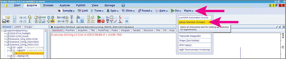
- While looking at your 1D 1H spectrum, go to the “Acquire” tab and pull down the “More” menu, then choose “Selective 1D experiments”.

1D NOESY setup 01 – menu
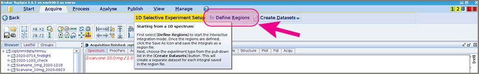
- A submenu will appear below your main buttons that includes a button labeled “Define Regions” Click that.
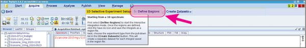
1D NOESY setup 02 – define excitation region(s)
- The Integration menu appears. Use the usual tools to “integrate” your peak(s) of interest.
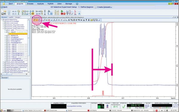
1D NOESY setup 03 – integrate
- Click the “Save-A” button, the “floppy-disk-with-an-A-on-it”. You get a menu that includes “Save integral regions to reg”. Click that.
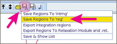
1D NOESY setup 04 – save region(s) to reg
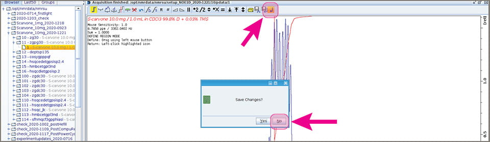
- Click the “return” button that does NOT have a floppy disk icon; answer “No” if it asks you to save the regions.
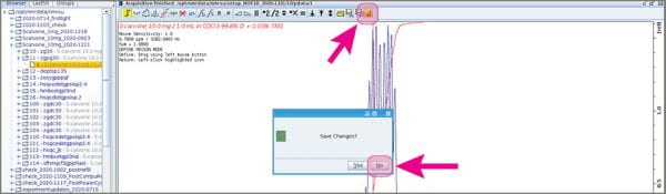
1D NOESY setup 05 – return and dont save
- Don’t do anything else. Go on to the next step

Step 3: Set up your experiments and start acquiring data
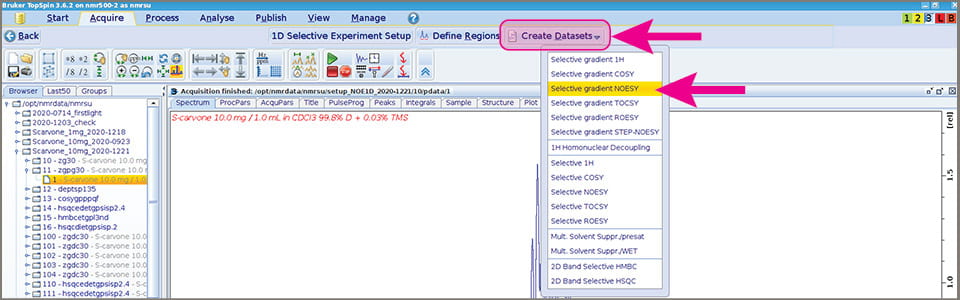
- Click the big “Create Datasets” button and choose “Selective gradient NOESY”.
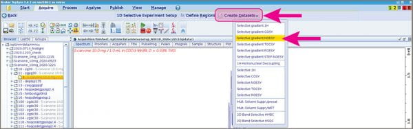
1D NOESY setup 06 – create NOESY experiment
- A popup window will appear that enables you to change your mixing time, increase the number of scans, and select the experiment number of your NOESY.
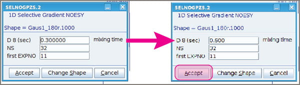
1D NOESY setup 07 – edit mixing time and NS
- The choice of mixing time is somewhat subjective. Details will follow soon in a blog post. Most small molecules do well with mixing times between ~0.5 and 0.8 sec.
- You may wish to increase NS, depending on how much material you have in your sample. NS needs to be a multiple of 2, but not a power of 2. For example, 38 is OK.
- Choose a spectrum number that will help you remember which spectrum (spectra) is the NOESY; I use “20”.
- Click “Accept” when you’re ready to move forward.
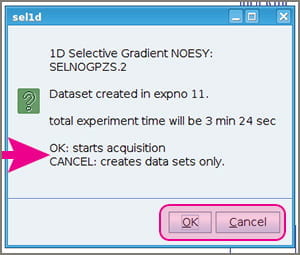
- A popup window will appear giving you a choice to either go ahead and start acquiring data (click OK), or simply let the experiment parameters be written to your experiment number and NOT proceed to acquiring data (Cancel). Clicking “Cancel” enables you to estimate the duration of your experiment, perhaps adjusting NS, D1, or other parameters.If you’re aiming for quantitative NOE and need a set of experiments with different mixing times for each peak, then you need to click “Cancel” at this stage so you can set up experiments with different D8 values.
1D NOESY setup 08 – choose to go or cancel
- If you clicked OK, you’re done! You should see the normal FID flash indicating data acquisition.
- If you clicked “Cancel”, maybe check your experiment time with “expt” or clicking the little square clock button. Adjust NS to what you’d like. Then do “RGA” and, when it’s done, “ZG”.
ALT: Exciting more than one peak
If you’re intending to examine more than one 1H atom, you need to set up a separate 1D NOE experiment for each one. Fortunately, this process is simple. In Step 2.3 above, simply integrate EACH peak you wish to excite. When you choose “Save regions to reg”, each region will be saved. When executing Step 3.3, choosing either “Ok” or “Cancel” will create spectrum folders for each of the 1D NOESY experiments – one for each excited peak. Be sure that, in Step 3.2, you choose a spectrum number that does not have any numbers above it already. For example, if you already have experiments “10” and “11”, choosing “12” is OK, but I’d still recommend “20” for clarity. If you have four peaks to excite, spectrum folders 20, 21, 22, and 23 will be created.
Analysis
Overview
When your spectrum is done acquiring, process it normally but adjust the phase so your excited peak is negative. It should be obviously the only major peak in the spectrum, much larger than everything else. Your NOE peaks will be positive and small.
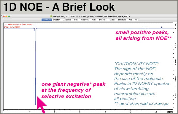
1D NOESY general features – one large negative peak and small positive NOE peaks
Closer Examination
A closer look along with molecular context may provide the best orientation (see figure below). Please note that MNova placed properly-numbered labels at the frequency of each assigned 1H frequency, which is very handy; the mechanics of making spectrum assignments in MNova will be covered in a future post. In this experiment, H#3 of S-carvone was selectively excited/inverted. The other peaks we observe come from magnetization that started on H#3 that then got transferred to other 1Hs via the 1H-1H NOE.
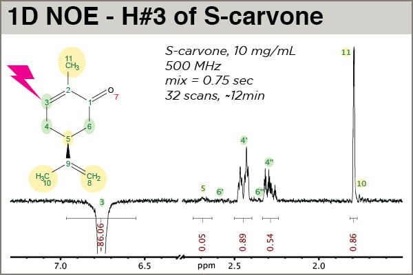
The 1D NOE spectrum resulting from excitation of H3 in carvone, employing 750 msec mixing time
One sees that the NOE peaks that appear strongest are for atoms closest to H3, the peak that was selectively inverted: H4′, H4”, and H11 (a methyl group). This experiment was done carefully enough (i.e., D1 allowed for complete relaxation between scans, and D8, the mixing time, was short enough that it falls within the linear range of NOE buildup for this atom) that the intensities are meaningful. H4” exhibits an NOE intensity just a little above half that of H4′, indicating 4” is slightly farther away. H11(methyl) is clearly closer to H3 than H10(methyl), which shows no significant NOE, helping confirm assignment. The small NOE observed for H5 is real, corresponding to a longer distnace than H3-H4′ or H3-H4”. This experiment should be run with significantly more scans (e.g., 128 or 256) to accurately measure the H3-H5 distance.
Note the values of the integrals. First, the untold story: prior to calibrating the integral areas here, another 1D NOESY had been run with identical parameters except D8 = 0.01 sec. This value is effectively zero, so the integral of the H3 peak, in arbitrary units, represents the “true” intensity of the peak before it has transferred its magnetization away via NOE. The peak in the spectrum above, with D8 = 0.75 sec, was normalized against the intensity of the other spectrum, and we observe that H3 has lost approximately 14% of its intensity by the end of the 0.75 sec mixing time. Thus calibrated, we can say the calibrated integral value of H4′, 0.89, represents a 0.89% NOE.
1D vs 2D NOESY
Critical comparison of 1D and 2D NOESY will be done in a later blog post. But for now, let’s consider the big picture:
1D NOESY experiments have some advantages over their 2D counterparts. 2D NOESY experiments reveal all the 1H-1H NOEs in a molecule at once, and are thus very good for determining 3D molecular structures. But they are usually time-consuming; the default 2D NOESY experiments on our 400 MHz spectrmeters takes a little over two hours to run. A 1D NOESY spectrum, however, can be set up and run manually in less than five minutes after a regular 1D 1H spectrum has been acquired.
Oftentimes, a chemical question can be answered very quickly with a 1D NOESY spectrum if it can be framed in the form “I need to determine which of two compounds I have; in compound #1, 1Hs A and B are closer than 4 or 5 Å, but in compound #2, they are too far to show NOE.” If you run a 1D NOESY spectrum and you see the key peak, you know you have compound #1. If you don’t see it, and you’ve verified that you’d taken enough scans that you should see it, then you can conclude you probably have compound #2.
Sometimes your question is better answered with a small set of 1D NOESY experiments. The tools in Topspin enable you to set up several 1D NOESY experiments to be run one after another, giving you one spectrum file each at the end. But if you’re querying more than five or six 1Hs, you’re probably better off with a 2D NOESY.
WRAP-UP
If you ever need to answer a structural question that knowing 1H-1H distances will help solve, pease consider the 1D NOESY expeirment. You don’t need special coaching or permission to run a 1D NOESY experiment, so you’re welcome to try it any time. Simply follow the instructions here or just showup at the spectrometer point your phone at the QR code, and follow along with the quick video. Enjoy!
Greetings.
Firstly, thank you for making such detailed yet easy to understand information about the NOESY experiments.
Secondly, where can I locate the post on the critical comparison between 1D and 2D NOESY.
Thanks!
Thanks! Unfortunately I haven’t gotten around to that post, so it’s still pending. They key issue is the choice the chemist has to make between 1D and 2D, and there are a number of factors involved, not all of which as technical.
– Resolution will be better in 1D, but that’s not strictly necessary if one’s peaks aren’t overlapped. 2D is necessary if a spectrum is congested with overlap. What I aim to show in that future post is a S/N comparison of 1D vs 2D for the same NOE crosspeak.
– Time often plays a factor. Our chemists can run walkup NMR with a 20 minute per visit time limit – not long enough for a 2D. Oftentimes they are simply interested in making a configurational assignment that can be answered with a single 1D NOE experiment they can run in 15 minutes. So then they’d choose 1D.
– Convenience. The chemist walking in to the lab faces the choice of whether to run a 1D NOE right away in walkup mode, as long as they can get everything done in 20 minutes, and get their answer immediately, OR submit their sample to the night queue of the autosampler for a 2D NOESY that gives them a result the next day.
– Cost. Because a 1D NOE takes much less time than a 2D, it’s cheaper. But if one needs a series of five or six 1D NOEs, is it worth it?
In any case, those are the sorts of things I’m aiming to address. Presenting an evidence-based approach to help the chemist choose between 1D and 2D based on a number of factors.
Thanks. – Josh
Hi Josh, thank you so much for the insight and clarification.
I think I understand better now.
So, I actually ran both 1D and 2D NOESY. I started with 2D but did not see the positive NOEs that I was sure I would see. Then, I did 1D and boom, could visualize even the weak peaks….#Thanks for the guidance in your article above.
Where I am stuck is, the positively phased peaks show NOEs with the excited peak right, but I can not seem to correlate them with the 1D proton spectrum where I did proton assignments. For the ones where I can sort off say is what I assigned, that positive NOE peak is at a different ppm than on the 1D proton spectrum.
I am not sure if I am making sense 🙂
Greetings.
Firstly, thank you for making such information!
Secondly, may I ask you a question? I wonder how to get a mixing time=0sec data because I wanna calculate the exchanging rate.
Forgive my poor English, thanks a million!